In the RVs with multiple instruments case study, we discussed fitting the radial velocity curve for a planetary system observed using multiple instruments. You might also want to fit data from multiple instruments when fitting the light curve of a transiting planet and that’s what we work through in this example. This is a somewhat more complicated example than the radial velocity case because some of the physical properties of the system can vary as as function of the instrument. Specifically, the transit depth (or the effective raduis of the planet) will be a function of the filter or effective wavelength of the observations. This is the idea behind transit spectroscopy and the method used in this case study could (and should!) be extended to that use case. In this case, we’ll combine the light curves from the Kepler and TESS missions for the planet host HAT-P-11.
Before getting into the details of this case study, let’s spend a minute talking about a topic that comes up a lot when discussing combining observations from different instruments or techniques. To many people, it seems intuitive that one should (and perhaps must) “weight” how much each dataset contributes to the likelihood based on how much they “trust” those data. For example, you might be worried that a dataset with more datapoints will have a larger effect on the the results than you would like. While this might seem intuitive, it’s wrong: the only way to combine datasets is to multiply their likelihood functions. Instead, it is useful to understand what you actually mean when you say that you don’t “trust” a dataset as much as another. What you’re really saying is that you don’t believe the observation model that you wrote down. For example, you might think that the quoted error bars are underestimated or there might be correlated noise that an uncorrelated normal observation model can’t capture. The benefit of thinking about it this way is that it suggests a solution to the problem: incorporate a more flexible observation model that can capture these issues. In this case study, the 4 years of (long-cadence) Kepler observations only include about two times as many data points as one month of TESS observations. But, as you can see in the figure below, these two datasets have different noise properties (both in terms of photon noise and correlated noise) so we will fit using a different flexible Gaussian process noise model for each data set that will take these different properties into account.
[3]:
import numpy as np
import lightkurve as lk
from astropy.io import fits
from collections import OrderedDict

kepler_lcfs = lk.search_lightcurve(
    "HAT-P-11", mission="Kepler", cadence="long"
).download_all(flux_column="pdcsap_flux")
kepler_lc = kepler_lcfs.stitch().remove_nans()
kepler_t = np.ascontiguousarray(kepler_lc.time.value, dtype=np.float64)
kepler_y = np.ascontiguousarray(1e3 * (kepler_lc.flux - 1), dtype=np.float64)
kepler_yerr = np.ascontiguousarray(1e3 * kepler_lc.flux_err, dtype=np.float64)

with fits.open(kepler_lcfs[0].filename) as hdu:
    hdr = hdu[1].header
kepler_texp = hdr["FRAMETIM"] * hdr["NUM_FRM"]
kepler_texp /= 60.0 * 60.0 * 24.0

tess_lcfs = lk.search_lightcurve(
    "HAT-P-11", mission="TESS", author="SPOC"
).download_all(flux_column="pdcsap_flux")
tess_lc = tess_lcfs.stitch().remove_nans()
tess_t = np.ascontiguousarray(
    tess_lc.time.value + 2457000 - 2454833, dtype=np.float64
)
tess_y = np.ascontiguousarray(1e3 * (tess_lc.flux - 1), dtype=np.float64)
tess_yerr = np.ascontiguousarray(1e3 * tess_lc.flux_err, dtype=np.float64)

with fits.open(tess_lcfs[0].filename) as hdu:
    hdr = hdu[1].header
tess_texp = hdr["FRAMETIM"] * hdr["NUM_FRM"]
tess_texp /= 60.0 * 60.0 * 24.0

datasets = OrderedDict(
    [
        ("Kepler", [kepler_t, kepler_y, kepler_yerr, kepler_texp]),
        ("TESS", [tess_t, tess_y, tess_yerr, tess_texp]),
    ]
)

fig, axes = plt.subplots(1, len(datasets), sharey=True, figsize=(10, 5))

for i, (name, (t, y, _, _)) in enumerate(datasets.items()):
    ax = axes[i]
    ax.plot(t, y, "k", lw=0.75, label=name)
    ax.set_xlabel("time [KBJD]")
    ax.set_title(name, fontsize=14)

    x_mid = 0.5 * (t.min() + t.max())
    ax.set_xlim(x_mid - 10, x_mid + 10)
axes[0].set_ylim(-10, 10)
fig.subplots_adjust(wspace=0.05)
_ = axes[0].set_ylabel("relative flux [ppt]")

This model is mostly the same as the one used in Quick fits for TESS light curves, but we’re allowing for different noise variances (both the white noise component and the GP amplitude), effective planet radii, and limb-darkening coeeficients for each dataset. For the purposes of demonstration, we’re sharing the length scale of the GP between the two datasets, but this could just have well been a different parameter for each dataset without changing the results. The
final change that we’re using is to use the approximate transit depth approx_depth (the depth of the transit at minimum assuming the limb-darkening profile is constant under the disk of the planet) as a parameter instead of the radius ratio. This does not have a large effect on the performance or the results, but it can sometimes be a useful parameterization when dealing with high signal-to-noise transits because it reduces the covariance between the radius parameter and the limb darkening
coefficients. As usual, we run a few iterations of sigma clipping and then find the maximum a posteriori parameters to check to make sure that everything is working:
[4]:
import pymc3 as pm
import pymc3_ext as pmx
import exoplanet as xo
import aesara_theano_fallback.tensor as tt
from functools import partial
from celerite2.theano import terms, GaussianProcess

# Period and reference transit time from the literature for initialization
lit_period = 4.887803076
lit_t0 = 124.8130808

# Find a reference transit time near the middle of the observations to avoid
# strong covariances between period and t0
x_min = min(np.min(x) for x, _, _, _ in datasets.values())
x_max = max(np.max(x) for x, _, _, _ in datasets.values())
x_mid = 0.5 * (x_min + x_max)
t0_ref = lit_t0 + lit_period * np.round((x_mid - lit_t0) / lit_period)

# Do several rounds of sigma clipping
for i in range(10):
    with pm.Model() as model:

        # Shared orbital parameters
        log_period = pm.Normal("log_period", mu=np.log(lit_period), sigma=1.0)
        period = pm.Deterministic("period", tt.exp(log_period))
        t0 = pm.Normal("t0", mu=t0_ref, sigma=1.0)
        log_dur = pm.Normal("log_dur", mu=np.log(0.1), sigma=10.0)
        dur = pm.Deterministic("dur", tt.exp(log_dur))
        b = pmx.UnitUniform("b")
        ld_arg = 1 - tt.sqrt(1 - b ** 2)
        orbit = xo.orbits.KeplerianOrbit(
            period=period, duration=dur, t0=t0, b=b
        )

        # We'll also say that the timescale of the GP will be shared
        rho_gp = pm.InverseGamma(
            "rho_gp",
            testval=2.0,
            **pmx.estimate_inverse_gamma_parameters(1.0, 5.0),
        )

        # Loop over the instruments
        parameters = dict()
        lc_models = dict()
        gp_preds = dict()
        gp_preds_with_mean = dict()
        for n, (name, (x, y, yerr, texp)) in enumerate(datasets.items()):

            # We define the per-instrument parameters in a submodel so that we
            # don't have to prefix the names manually
            with pm.Model(name=name, model=model):
                # The flux zero point
                mean = pm.Normal("mean", mu=0.0, sigma=10.0)

                # The limb darkening
                u = xo.QuadLimbDark("u")
                star = xo.LimbDarkLightCurve(u)

                # The radius ratio
                log_approx_depth = pm.Normal(
                    "log_approx_depth", mu=np.log(4e-3), sigma=10
                )
                ld = 1 - u[0] * ld_arg - u[1] * ld_arg ** 2
                ror = pm.Deterministic(
                    "ror", tt.exp(0.5 * log_approx_depth) / tt.sqrt(ld)
                )

                # Noise parameters
                med_yerr = np.median(yerr)
                std = np.std(y)
                sigma = pm.InverseGamma(
                    "sigma",
                    testval=med_yerr,
                    **pmx.estimate_inverse_gamma_parameters(
                        med_yerr, 0.5 * std
                    ),
                )
                sigma_gp = pm.InverseGamma(
                    "sigma_gp",
                    testval=0.5 * std,
                    **pmx.estimate_inverse_gamma_parameters(
                        med_yerr, 0.5 * std
                    ),
                )

                # Keep track of the parameters for optimization
                parameters[name] = [mean, u, log_approx_depth]
                parameters[f"{name}_noise"] = [sigma, sigma_gp]

            # The light curve model
            def lc_model(mean, star, ror, texp, t):
                return mean + 1e3 * tt.sum(
                    star.get_light_curve(orbit=orbit, r=ror, t=t, texp=texp),
                    axis=-1,
                )

            lc_model = partial(lc_model, mean, star, ror, texp)
            lc_models[name] = lc_model

            # The Gaussian Process noise model
            kernel = terms.SHOTerm(sigma=sigma_gp, rho=rho_gp, Q=1.0 / 3)
            gp = GaussianProcess(
                kernel, t=x, diag=yerr ** 2 + sigma ** 2, mean=lc_model
            )
            gp.marginal(f"{name}_obs", observed=y)
            gp_preds[name] = gp.predict(y, include_mean=False)
            gp_preds_with_mean[name] = gp_preds[name] + gp.mean_value

        # Optimize the model
        map_soln = model.test_point
        for name in datasets:
            map_soln = pmx.optimize(map_soln, parameters[name])
        for name in datasets:
            map_soln = pmx.optimize(map_soln, parameters[f"{name}_noise"])
            map_soln = pmx.optimize(map_soln, parameters[name] + [log_dur, b])
        map_soln = pmx.optimize(map_soln)

        # Do some sigma clipping
        num = dict((name, len(datasets[name][0])) for name in datasets)
        clipped = dict()
        masks = dict()
        for name in datasets:
            mdl = pmx.eval_in_model(gp_preds_with_mean[name], map_soln)
            resid = datasets[name][1] - mdl
            sigma = np.sqrt(np.median((resid - np.median(resid)) ** 2))
            masks[name] = np.abs(resid - np.median(resid)) < 7 * sigma
            clipped[name] = num[name] - masks[name].sum()
            print(f"Sigma clipped {clipped[name]} {name} light curve points")

        if all(c < 10 for c in clipped.values()):
            break

        else:
            for name in datasets:
                datasets[name][0] = datasets[name][0][masks[name]]
                datasets[name][1] = datasets[name][1][masks[name]]
                datasets[name][2] = datasets[name][2][masks[name]]
/home/runner/work/case-studies/case-studies/src/exoplanet/src/exoplanet/orbits/keplerian.py:110: UserWarning: When using the 'duration' parameter in KeplerianOrbit, the 'ror' parameter should also be provided.
  warnings.warn(
optimizing logp for variables: [Kepler_log_approx_depth, Kepler_u, Kepler_mean]
message: Desired error not necessarily achieved due to precision loss.
logp: -24191.163749048814 -> 5802.310351878092
optimizing logp for variables: [TESS_log_approx_depth, TESS_u, TESS_mean]
message: Desired error not necessarily achieved due to precision loss.
logp: 5802.310351878092 -> 6099.7319783094645
optimizing logp for variables: [Kepler_sigma_gp, Kepler_sigma]
message: Optimization terminated successfully.
logp: 6099.7319783094645 -> 16460.578209989704
optimizing logp for variables: [b, log_dur, Kepler_log_approx_depth, Kepler_u, Kepler_mean]
message: Optimization terminated successfully.
logp: 16460.57820998969 -> 19952.20237321892
optimizing logp for variables: [TESS_sigma_gp, TESS_sigma]
message: Optimization terminated successfully.
logp: 19952.202373218905 -> 20448.483886076916
optimizing logp for variables: [b, log_dur, TESS_log_approx_depth, TESS_u, TESS_mean]
message: Desired error not necessarily achieved due to precision loss.
logp: 20448.48388607693 -> 20544.7411963084
optimizing logp for variables: [TESS_sigma_gp, TESS_sigma, TESS_log_approx_depth, TESS_u, TESS_mean, Kepler_sigma_gp, Kepler_sigma, Kepler_log_approx_depth, Kepler_u, Kepler_mean, rho_gp, b, log_dur, t0, log_period]
message: Desired error not necessarily achieved due to precision loss.
logp: 20544.7411963084 -> 27342.533952675403
Sigma clipped 337 Kepler light curve points
Sigma clipped 24 TESS light curve points
/home/runner/work/case-studies/case-studies/src/exoplanet/src/exoplanet/orbits/keplerian.py:110: UserWarning: When using the 'duration' parameter in KeplerianOrbit, the 'ror' parameter should also be provided.
  warnings.warn(
optimizing logp for variables: [Kepler_log_approx_depth, Kepler_u, Kepler_mean]
message: Desired error not necessarily achieved due to precision loss.
logp: -10421.336128852028 -> 19381.93181392811
optimizing logp for variables: [TESS_log_approx_depth, TESS_u, TESS_mean]
message: Optimization terminated successfully.
logp: 19381.93181392811 -> 19684.999895527624
optimizing logp for variables: [Kepler_sigma_gp, Kepler_sigma]
message: Optimization terminated successfully.
logp: 19684.999895527624 -> 27940.899208534967
optimizing logp for variables: [b, log_dur, Kepler_log_approx_depth, Kepler_u, Kepler_mean]
message: Desired error not necessarily achieved due to precision loss.
logp: 27940.899208534982 -> 32897.27501143553
optimizing logp for variables: [TESS_sigma_gp, TESS_sigma]
message: Desired error not necessarily achieved due to precision loss.
logp: 32897.275011435566 -> 33474.448303035446
optimizing logp for variables: [b, log_dur, TESS_log_approx_depth, TESS_u, TESS_mean]
message: Desired error not necessarily achieved due to precision loss.
logp: 33474.44830303542 -> 33566.758220623684
optimizing logp for variables: [TESS_sigma_gp, TESS_sigma, TESS_log_approx_depth, TESS_u, TESS_mean, Kepler_sigma_gp, Kepler_sigma, Kepler_log_approx_depth, Kepler_u, Kepler_mean, rho_gp, b, log_dur, t0, log_period]
message: Desired error not necessarily achieved due to precision loss.
logp: 33566.758220623684 -> 42251.83421721451
Sigma clipped 27 Kepler light curve points
Sigma clipped 0 TESS light curve points
/home/runner/work/case-studies/case-studies/src/exoplanet/src/exoplanet/orbits/keplerian.py:110: UserWarning: When using the 'duration' parameter in KeplerianOrbit, the 'ror' parameter should also be provided.
  warnings.warn(
optimizing logp for variables: [Kepler_log_approx_depth, Kepler_u, Kepler_mean]
message: Desired error not necessarily achieved due to precision loss.
logp: -10165.132305951134 -> 19585.89154889733
optimizing logp for variables: [TESS_log_approx_depth, TESS_u, TESS_mean]
message: Optimization terminated successfully.
logp: 19585.89154889733 -> 19888.959630496676
optimizing logp for variables: [Kepler_sigma_gp, Kepler_sigma]
message: Desired error not necessarily achieved due to precision loss.
logp: 19888.959630496676 -> 28166.57351327523
optimizing logp for variables: [b, log_dur, Kepler_log_approx_depth, Kepler_u, Kepler_mean]
message: Optimization terminated successfully.
logp: 28166.573513275296 -> 33141.23604655786
optimizing logp for variables: [TESS_sigma_gp, TESS_sigma]
message: Desired error not necessarily achieved due to precision loss.
logp: 33141.23604655789 -> 33719.09614865158
optimizing logp for variables: [b, log_dur, TESS_log_approx_depth, TESS_u, TESS_mean]
message: Desired error not necessarily achieved due to precision loss.
logp: 33719.09614865156 -> 33808.074520073555
optimizing logp for variables: [TESS_sigma_gp, TESS_sigma, TESS_log_approx_depth, TESS_u, TESS_mean, Kepler_sigma_gp, Kepler_sigma, Kepler_log_approx_depth, Kepler_u, Kepler_mean, rho_gp, b, log_dur, t0, log_period]
message: Desired error not necessarily achieved due to precision loss.
logp: 33808.074520073555 -> 42562.00722107063
Sigma clipped 5 Kepler light curve points
Sigma clipped 0 TESS light curve points
Here are the two phased light curves (with the Gaussian process model removed). We can see the effect of exposure time integration and the difference in photometric precision, but everything should be looking good!
[5]:
dt = np.linspace(-0.2, 0.2, 500)

with model:
    trends = pmx.eval_in_model([gp_preds[k] for k in datasets], map_soln)
    phase_curves = pmx.eval_in_model(
        [lc_models[k](t0 + dt) for k in datasets], map_soln
    )

fig, axes = plt.subplots(2, sharex=True, sharey=True, figsize=(8, 6))

for n, name in enumerate(datasets):
    ax = axes[n]

    x, y = datasets[name][:2]

    period = map_soln["period"]
    folded = (x - map_soln["t0"] + 0.5 * period) % period - 0.5 * period
    m = np.abs(folded) < 0.2
    ax.plot(
        folded[m],
        (y - trends[n] - map_soln[f"{name}_mean"])[m],
        ".k",
        alpha=0.3,
        mec="none",
    )
    ax.plot(
        dt, phase_curves[n] - map_soln[f"{name}_mean"], f"C{n}", label=name
    )
    ax.annotate(
        name,
        xy=(1, 0),
        xycoords="axes fraction",
        va="bottom",
        ha="right",
        xytext=(-3, 3),
        textcoords="offset points",
        fontsize=14,
    )

axes[-1].set_xlim(-0.15, 0.15)
axes[-1].set_xlabel("time since transit [days]")
for ax in axes:
    ax.set_ylabel("relative flux [ppt]")
Then we run the MCMC:
[6]:
np.random.seed(11)
with model:
    trace = pmx.sample(
        tune=2500,
        draws=2000,
        start=map_soln,
        cores=2,
        chains=2,
        initial_accept=0.5,
        target_accept=0.95,
        return_inferencedata=True,
    )
Multiprocess sampling (2 chains in 2 jobs)
NUTS: [TESS_sigma_gp, TESS_sigma, TESS_log_approx_depth, TESS_u, TESS_mean, Kepler_sigma_gp, Kepler_sigma, Kepler_log_approx_depth, Kepler_u, Kepler_mean, rho_gp, b, log_dur, t0, log_period]
Sampling 2 chains for 2_500 tune and 2_000 draw iterations (5_000 + 4_000 draws total) took 2160 seconds.
And check the convergence diagnostics:
[7]:
import arviz as az

az.summary(trace)
[7]:
| mean | sd | hdi_3% | hdi_97% | mcse_mean | mcse_sd | ess_bulk | ess_tail | r_hat | |
|---|---|---|---|---|---|---|---|---|---|
| log_period | 1.587 | 0.000 | 1.587 | 1.587 | 0.000 | 0.000 | 6759.0 | 2551.0 | 1.0 |
| t0 | 2011.505 | 0.000 | 2011.505 | 2011.505 | 0.000 | 0.000 | 6363.0 | 2966.0 | 1.0 |
| log_dur | -2.388 | 0.002 | -2.392 | -2.386 | 0.000 | 0.000 | 1858.0 | 1697.0 | 1.0 |
| Kepler_mean | -0.331 | 0.195 | -0.678 | 0.046 | 0.002 | 0.002 | 7427.0 | 2864.0 | 1.0 |
| Kepler_log_approx_depth | -5.685 | 0.002 | -5.689 | -5.681 | 0.000 | 0.000 | 4620.0 | 3009.0 | 1.0 |
| TESS_mean | -0.033 | 0.171 | -0.343 | 0.298 | 0.002 | 0.003 | 6074.0 | 3013.0 | 1.0 |
| TESS_log_approx_depth | -5.671 | 0.012 | -5.694 | -5.648 | 0.000 | 0.000 | 4608.0 | 3233.0 | 1.0 |
| period | 4.888 | 0.000 | 4.888 | 4.888 | 0.000 | 0.000 | 6759.0 | 2551.0 | 1.0 |
| dur | 0.092 | 0.000 | 0.091 | 0.092 | 0.000 | 0.000 | 1858.0 | 1697.0 | 1.0 |
| b | 0.407 | 0.038 | 0.338 | 0.478 | 0.001 | 0.001 | 2072.0 | 1546.0 | 1.0 |
| rho_gp | 6.017 | 0.087 | 5.859 | 6.187 | 0.001 | 0.001 | 7020.0 | 2196.0 | 1.0 |
| Kepler_u[0] | 0.720 | 0.017 | 0.688 | 0.753 | 0.000 | 0.000 | 1799.0 | 1771.0 | 1.0 |
| Kepler_u[1] | -0.114 | 0.031 | -0.175 | -0.059 | 0.001 | 0.001 | 1852.0 | 1948.0 | 1.0 |
| Kepler_ror | 0.060 | 0.000 | 0.060 | 0.061 | 0.000 | 0.000 | 1882.0 | 1538.0 | 1.0 |
| Kepler_sigma | 0.027 | 0.000 | 0.027 | 0.027 | 0.000 | 0.000 | 6715.0 | 2823.0 | 1.0 |
| Kepler_sigma_gp | 2.776 | 0.055 | 2.670 | 2.879 | 0.001 | 0.000 | 6759.0 | 2738.0 | 1.0 |
| TESS_u[0] | 0.649 | 0.101 | 0.461 | 0.829 | 0.002 | 0.002 | 1962.0 | 2095.0 | 1.0 |
| TESS_u[1] | -0.180 | 0.139 | -0.408 | 0.069 | 0.003 | 0.002 | 1777.0 | 1559.0 | 1.0 |
| TESS_ror | 0.060 | 0.000 | 0.060 | 0.061 | 0.000 | 0.000 | 2560.0 | 2497.0 | 1.0 |
| TESS_sigma | 0.384 | 0.004 | 0.377 | 0.391 | 0.000 | 0.000 | 8171.0 | 2563.0 | 1.0 |
| TESS_sigma_gp | 0.557 | 0.014 | 0.530 | 0.584 | 0.000 | 0.000 | 6926.0 | 2283.0 | 1.0 |
Since we fit for a radius ratio in each band, we can see if the transit depth is different in Kepler compared to TESS. The plot below demonstrates that there is no statistically significant difference between the radii measured in these two bands:
[8]:
plt.hist(
    trace.posterior["Kepler_ror"].values.flatten(),
    30,
    density=True,
    histtype="step",
    label="Kepler",
)
plt.hist(
    trace.posterior["TESS_ror"].values.flatten(),
    30,
    density=True,
    histtype="step",
    label="TESS",
)
plt.yticks([])
plt.xlabel("effective radius ratio")
_ = plt.legend(fontsize=12)

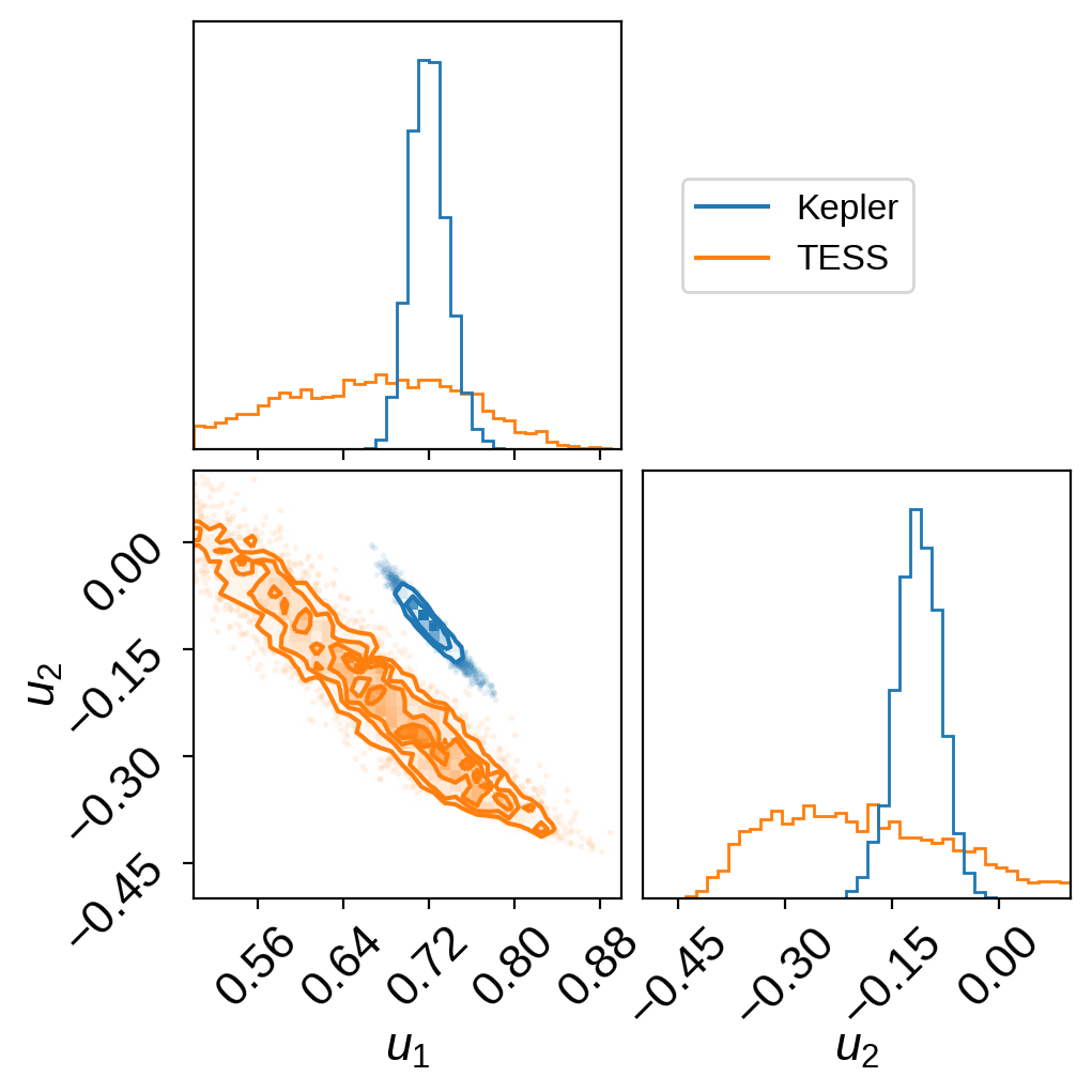
We can also compare the inferred limb-darkening coefficients:
[9]:
import corner

fig = corner.corner(
    trace,
    var_names=["TESS_u"],
    bins=40,
    color="C1",
    range=((0.5, 0.9), (-0.5, 0.1)),
)
corner.corner(
    trace,
    var_names=["Kepler_u"],
    bins=40,
    color="C0",
    fig=fig,
    labels=["$u_1$", "$u_2$"],
    range=((0.5, 0.9), (-0.5, 0.1)),
)
fig.axes[0].axvline(-1.0, color="C0", label="Kepler")
fig.axes[0].axvline(-1.0, color="C1", label="TESS")
_ = fig.axes[0].legend(
    fontsize=12, loc="center left", bbox_to_anchor=(1.1, 0.5)
)
As described in the citation tutorial, we can use citations.get_citations_for_model to construct an acknowledgement and BibTeX listing that includes the relevant citations for this model.
[10]:
with model:
    txt, bib = xo.citations.get_citations_for_model()
print(txt)
This research made use of \textsf{exoplanet} \citep{exoplanet} and its
dependencies \citep{celerite2:foremanmackey17, celerite2:foremanmackey18,
exoplanet:arviz, exoplanet:astropy13, exoplanet:astropy18, exoplanet:pymc3,
exoplanet:theano}.
[11]:
print("\n".join(bib.splitlines()[:10]) + "\n...")
@misc{exoplanet,
  author = {Daniel Foreman-Mackey and Arjun Savel and Rodrigo Luger  and
            Eric Agol and Ian Czekala and Adrian Price-Whelan and
            Christina Hedges and Emily Gilbert and Luke Bouma and Tom Barclay
            and Timothy D. Brandt},
   title = {exoplanet-dev/exoplanet v0.5.0},
   month = may,
    year = 2021,
     doi = {10.5281/zenodo.1998447},
...