In this tutorial, we will reproduce the fits to the transiting planet in the Pi Mensae system discovered by Huang et al. (2018). The data processing and model are similar to the Putting it all together case study, but with a few extra bits like aperture selection and de-trending.
To start, we need to download the target pixel file:
[3]:
import numpy as np
import lightkurve as lk
import matplotlib.pyplot as plt

lc_file = lk.search_lightcurvefile("TIC 261136679", sector=1).download(
    quality_bitmask="hardest"
)
lc = lc_file.PDCSAP_FLUX.remove_nans().normalize().remove_outliers()
time = lc.time
flux = lc.flux
m = lc.quality == 0
with lc_file.hdu as hdu:
    hdr = hdu[1].header

texp = hdr["FRAMETIM"] * hdr["NUM_FRM"]
texp /= 60.0 * 60.0 * 24.0

ref_time = 0.5 * (np.min(time) + np.max(time))
x = np.ascontiguousarray(time[m] - ref_time, dtype=np.float64)
y = np.ascontiguousarray(1e3 * (flux[m] - 1.0), dtype=np.float64)

plt.plot(x, y, ".k")
plt.xlabel("time [days]")
plt.ylabel("relative flux [ppt]")
_ = plt.xlim(x.min(), x.max())

Now, let’s use the box least squares periodogram from AstroPy (Note: you’ll need AstroPy v3.1 or more recent to use this feature) to estimate the period, phase, and depth of the transit.
[4]:
from astropy.timeseries import BoxLeastSquares

period_grid = np.exp(np.linspace(np.log(1), np.log(15), 50000))

bls = BoxLeastSquares(x, y)
bls_power = bls.power(period_grid, 0.1, oversample=20)

# Save the highest peak as the planet candidate
index = np.argmax(bls_power.power)
bls_period = bls_power.period[index]
bls_t0 = bls_power.transit_time[index]
bls_depth = bls_power.depth[index]
transit_mask = bls.transit_mask(x, bls_period, 0.2, bls_t0)

fig, axes = plt.subplots(2, 1, figsize=(10, 10))

# Plot the periodogram
ax = axes[0]
ax.axvline(np.log10(bls_period), color="C1", lw=5, alpha=0.8)
ax.plot(np.log10(bls_power.period), bls_power.power, "k")
ax.annotate(
    "period = {0:.4f} d".format(bls_period),
    (0, 1),
    xycoords="axes fraction",
    xytext=(5, -5),
    textcoords="offset points",
    va="top",
    ha="left",
    fontsize=12,
)
ax.set_ylabel("bls power")
ax.set_yticks([])
ax.set_xlim(np.log10(period_grid.min()), np.log10(period_grid.max()))
ax.set_xlabel("log10(period)")

# Plot the folded transit
ax = axes[1]
x_fold = (x - bls_t0 + 0.5 * bls_period) % bls_period - 0.5 * bls_period
m = np.abs(x_fold) < 0.4
ax.plot(x_fold[m], y[m], ".k")

# Overplot the phase binned light curve
bins = np.linspace(-0.41, 0.41, 32)
denom, _ = np.histogram(x_fold, bins)
num, _ = np.histogram(x_fold, bins, weights=y)
denom[num == 0] = 1.0
ax.plot(0.5 * (bins[1:] + bins[:-1]), num / denom, color="C1")

ax.set_xlim(-0.3, 0.3)
ax.set_ylabel("de-trended flux [ppt]")
_ = ax.set_xlabel("time since transit")

The transit model, initialization, and sampling are all nearly the same as the one in Putting it all together.
[5]:
import exoplanet as xo
import pymc3 as pm
import theano.tensor as tt

import pymc3_ext as pmx
from celerite2.theano import terms, GaussianProcess


def build_model(mask=None, start=None):
    if mask is None:
        mask = np.ones(len(x), dtype=bool)
    with pm.Model() as model:

        # Parameters for the stellar properties
        mean = pm.Normal("mean", mu=0.0, sd=10.0)
        u_star = xo.QuadLimbDark("u_star")

        # Stellar parameters from Huang et al (2018)
        M_star_huang = 1.094, 0.039
        R_star_huang = 1.10, 0.023
        BoundedNormal = pm.Bound(pm.Normal, lower=0, upper=3)
        m_star = BoundedNormal(
            "m_star", mu=M_star_huang[0], sd=M_star_huang[1]
        )
        r_star = BoundedNormal(
            "r_star", mu=R_star_huang[0], sd=R_star_huang[1]
        )

        # Orbital parameters for the planets
        period = pm.Lognormal("period", mu=np.log(bls_period), sd=1)
        t0 = pm.Normal("t0", mu=bls_t0, sd=1)
        r_pl = pm.Lognormal(
            "r_pl",
            sd=1.0,
            mu=0.5 * np.log(1e-3 * np.array(bls_depth))
            + np.log(R_star_huang[0]),
        )
        ror = pm.Deterministic("ror", r_pl / r_star)
        b = xo.distributions.ImpactParameter("b", ror=ror)

        ecs = pmx.UnitDisk("ecs", testval=np.array([0.01, 0.0]))
        ecc = pm.Deterministic("ecc", tt.sum(ecs ** 2))
        omega = pm.Deterministic("omega", tt.arctan2(ecs[1], ecs[0]))
        xo.eccentricity.kipping13("ecc_prior", fixed=True, observed=ecc)

        # Transit jitter & GP parameters
        sigma_lc = pm.Lognormal("sigma_lc", mu=np.log(np.std(y[mask])), sd=10)
        rho_gp = pm.Lognormal("rho_gp", mu=0, sd=10)
        sigma_gp = pm.Lognormal("sigma_gp", mu=np.log(np.std(y[mask])), sd=10)

        # Orbit model
        orbit = xo.orbits.KeplerianOrbit(
            r_star=r_star,
            m_star=m_star,
            period=period,
            t0=t0,
            b=b,
            ecc=ecc,
            omega=omega,
        )

        # Compute the model light curve
        light_curves = pm.Deterministic(
            "light_curves",
            xo.LimbDarkLightCurve(u_star).get_light_curve(
                orbit=orbit, r=r_pl, t=x[mask], texp=texp
            )
            * 1e3,
        )
        light_curve = tt.sum(light_curves, axis=-1) + mean
        resid = y[mask] - light_curve

        # GP model for the light curve
        kernel = terms.SHOTerm(sigma=sigma_gp, rho=rho_gp, Q=1 / np.sqrt(2))
        gp = GaussianProcess(kernel, t=x[mask], yerr=sigma_lc)
        gp.marginal("gp", observed=resid)
        pm.Deterministic("gp_pred", gp.predict(resid))

        # Fit for the maximum a posteriori parameters, I've found that I can get
        # a better solution by trying different combinations of parameters in turn
        if start is None:
            start = model.test_point
        map_soln = pmx.optimize(start=start, vars=[sigma_lc, sigma_gp, rho_gp])
        map_soln = pmx.optimize(start=map_soln, vars=[r_pl])
        map_soln = pmx.optimize(start=map_soln, vars=[b])
        map_soln = pmx.optimize(start=map_soln, vars=[period, t0])
        map_soln = pmx.optimize(start=map_soln, vars=[u_star])
        map_soln = pmx.optimize(start=map_soln, vars=[r_pl])
        map_soln = pmx.optimize(start=map_soln, vars=[b])
        map_soln = pmx.optimize(start=map_soln, vars=[ecs])
        map_soln = pmx.optimize(start=map_soln, vars=[mean])
        map_soln = pmx.optimize(
            start=map_soln, vars=[sigma_lc, sigma_gp, rho_gp]
        )
        map_soln = pmx.optimize(start=map_soln)

    return model, map_soln


model0, map_soln0 = build_model()
optimizing logp for variables: [rho_gp, sigma_gp, sigma_lc]
message: Desired error not necessarily achieved due to precision loss.
logp: 362.5039496547229 -> 699.7041405471658
optimizing logp for variables: [r_pl]
message: Optimization terminated successfully.
logp: 699.7041405471695 -> 700.7459969473945
optimizing logp for variables: [b, r_pl, r_star]
message: Optimization terminated successfully.
logp: 700.7459969473945 -> 874.8144918706691
optimizing logp for variables: [t0, period]
message: Desired error not necessarily achieved due to precision loss.
logp: 874.8144918706673 -> 877.207170521714
optimizing logp for variables: [u_star]
message: Optimization terminated successfully.
logp: 877.2071705217104 -> 877.6030372944554
optimizing logp for variables: [r_pl]
message: Optimization terminated successfully.
logp: 877.6030372944517 -> 877.6770071323643
optimizing logp for variables: [b, r_pl, r_star]
message: Optimization terminated successfully.
logp: 877.6770071323643 -> 877.749603133638
optimizing logp for variables: [ecs]
message: Optimization terminated successfully.
logp: 877.749603133638 -> 878.3326077948664
optimizing logp for variables: [mean]
message: Optimization terminated successfully.
logp: 878.3326077948645 -> 879.9061415721907
optimizing logp for variables: [rho_gp, sigma_gp, sigma_lc]
message: Optimization terminated successfully.
logp: 879.9061415721907 -> 880.0638635276545
optimizing logp for variables: [sigma_gp, rho_gp, sigma_lc, ecs, b, r_pl, t0, period, r_star, m_star, u_star, mean]
message: Desired error not necessarily achieved due to precision loss.
logp: 880.0638635276581 -> 935.2849116034278
Here’s how we plot the initial light curve model:
[6]:
def plot_light_curve(soln, mask=None):
    if mask is None:
        mask = np.ones(len(x), dtype=bool)

    fig, axes = plt.subplots(3, 1, figsize=(10, 7), sharex=True)

    ax = axes[0]
    ax.plot(x[mask], y[mask], "k", label="data")
    gp_mod = soln["gp_pred"] + soln["mean"]
    ax.plot(x[mask], gp_mod, color="C2", label="gp model")
    ax.legend(fontsize=10)
    ax.set_ylabel("relative flux [ppt]")

    ax = axes[1]
    ax.plot(x[mask], y[mask] - gp_mod, "k", label="de-trended data")
    for i, l in enumerate("b"):
        mod = soln["light_curves"][:, i]
        ax.plot(x[mask], mod, label="planet {0}".format(l))
    ax.legend(fontsize=10, loc=3)
    ax.set_ylabel("de-trended flux [ppt]")

    ax = axes[2]
    mod = gp_mod + np.sum(soln["light_curves"], axis=-1)
    ax.plot(x[mask], y[mask] - mod, "k")
    ax.axhline(0, color="#aaaaaa", lw=1)
    ax.set_ylabel("residuals [ppt]")
    ax.set_xlim(x[mask].min(), x[mask].max())
    ax.set_xlabel("time [days]")

    return fig


_ = plot_light_curve(map_soln0)

As in Putting it all together, we can do some sigma clipping to remove significant outliers.
[7]:
mod = (
    map_soln0["gp_pred"]
    + map_soln0["mean"]
    + np.sum(map_soln0["light_curves"], axis=-1)
)
resid = y - mod
rms = np.sqrt(np.median(resid ** 2))
mask = np.abs(resid) < 5 * rms

plt.figure(figsize=(10, 5))
plt.plot(x, resid, "k", label="data")
plt.plot(x[~mask], resid[~mask], "xr", label="outliers")
plt.axhline(0, color="#aaaaaa", lw=1)
plt.ylabel("residuals [ppt]")
plt.xlabel("time [days]")
plt.legend(fontsize=12, loc=3)
_ = plt.xlim(x.min(), x.max())

And then we re-build the model using the data without outliers.
[8]:
model, map_soln = build_model(mask, map_soln0)
_ = plot_light_curve(map_soln, mask)
optimizing logp for variables: [rho_gp, sigma_gp, sigma_lc]
message: Optimization terminated successfully.
logp: 2218.3946391081895 -> 2324.654909137419
optimizing logp for variables: [r_pl]
message: Optimization terminated successfully.
logp: 2324.65490913741 -> 2324.6704029831053
optimizing logp for variables: [b, r_pl, r_star]
message: Optimization terminated successfully.
logp: 2324.6704029831053 -> 2324.6729081040767
optimizing logp for variables: [t0, period]
message: Desired error not necessarily achieved due to precision loss.
logp: 2324.672908104075 -> 2324.6770116795547
optimizing logp for variables: [u_star]
message: Optimization terminated successfully.
logp: 2324.6770116795474 -> 2324.745321767219
optimizing logp for variables: [r_pl]
message: Optimization terminated successfully.
logp: 2324.7453217672173 -> 2324.7453263422813
optimizing logp for variables: [b, r_pl, r_star]
message: Optimization terminated successfully.
logp: 2324.7453263422813 -> 2324.748426829486
optimizing logp for variables: [ecs]
message: Optimization terminated successfully.
logp: 2324.7484268294843 -> 2324.7484421765657
optimizing logp for variables: [mean]
message: Optimization terminated successfully.
logp: 2324.748442176562 -> 2324.7562105257725
optimizing logp for variables: [rho_gp, sigma_gp, sigma_lc]
message: Optimization terminated successfully.
logp: 2324.7562105257725 -> 2324.756483900992
optimizing logp for variables: [sigma_gp, rho_gp, sigma_lc, ecs, b, r_pl, t0, period, r_star, m_star, u_star, mean]
message: Desired error not necessarily achieved due to precision loss.
logp: 2324.7564839009938 -> 2324.757330464715

Now that we have the model, we can sample:
[9]:
np.random.seed(261136679)
with model:
    trace = pmx.sample(
        tune=2500,
        draws=2000,
        start=map_soln,
        cores=2,
        chains=2,
        initial_accept=0.8,
        target_accept=0.95,
    )
Multiprocess sampling (2 chains in 2 jobs)
NUTS: [sigma_gp, rho_gp, sigma_lc, ecs, b, r_pl, t0, period, r_star, m_star, u_star, mean]
Sampling 2 chains for 2_500 tune and 2_000 draw iterations (5_000 + 4_000 draws total) took 2149 seconds.
[10]:
with model:
    summary = pm.summary(
        trace,
        var_names=[
            "omega",
            "ecc",
            "r_pl",
            "b",
            "t0",
            "period",
            "r_star",
            "m_star",
            "u_star",
            "mean",
        ],
    )
summary
[10]:
| mean | sd | hdi_3% | hdi_97% | mcse_mean | mcse_sd | ess_mean | ess_sd | ess_bulk | ess_tail | r_hat | |
|---|---|---|---|---|---|---|---|---|---|---|---|
| omega | 0.339 | 1.852 | -2.837 | 3.140 | 0.041 | 0.029 | 2044.0 | 2044.0 | 2333.0 | 2969.0 | 1.0 |
| ecc | 0.217 | 0.154 | 0.000 | 0.507 | 0.004 | 0.003 | 1438.0 | 1304.0 | 1719.0 | 1771.0 | 1.0 |
| r_pl | 0.016 | 0.001 | 0.014 | 0.019 | 0.000 | 0.000 | 2516.0 | 2466.0 | 2625.0 | 2595.0 | 1.0 |
| b | 0.473 | 0.215 | 0.018 | 0.776 | 0.006 | 0.004 | 1171.0 | 1171.0 | 1176.0 | 1264.0 | 1.0 |
| t0 | -13.730 | 0.003 | -13.737 | -13.724 | 0.000 | 0.000 | 3082.0 | 3082.0 | 3261.0 | 2097.0 | 1.0 |
| period | 6.266 | 0.001 | 6.264 | 6.269 | 0.000 | 0.000 | 3669.0 | 3669.0 | 3753.0 | 2096.0 | 1.0 |
| r_star | 1.099 | 0.023 | 1.058 | 1.143 | 0.000 | 0.000 | 4994.0 | 4994.0 | 4995.0 | 2987.0 | 1.0 |
| m_star | 1.095 | 0.039 | 1.025 | 1.170 | 0.001 | 0.000 | 5013.0 | 5013.0 | 5004.0 | 2965.0 | 1.0 |
| u_star[0] | 0.554 | 0.371 | 0.000 | 1.197 | 0.006 | 0.004 | 3804.0 | 3596.0 | 3398.0 | 2116.0 | 1.0 |
| u_star[1] | 0.169 | 0.392 | -0.494 | 0.887 | 0.006 | 0.006 | 4142.0 | 2381.0 | 3872.0 | 2664.0 | 1.0 |
| mean | 0.021 | 0.012 | -0.000 | 0.044 | 0.000 | 0.000 | 4833.0 | 4096.0 | 4840.0 | 3116.0 | 1.0 |
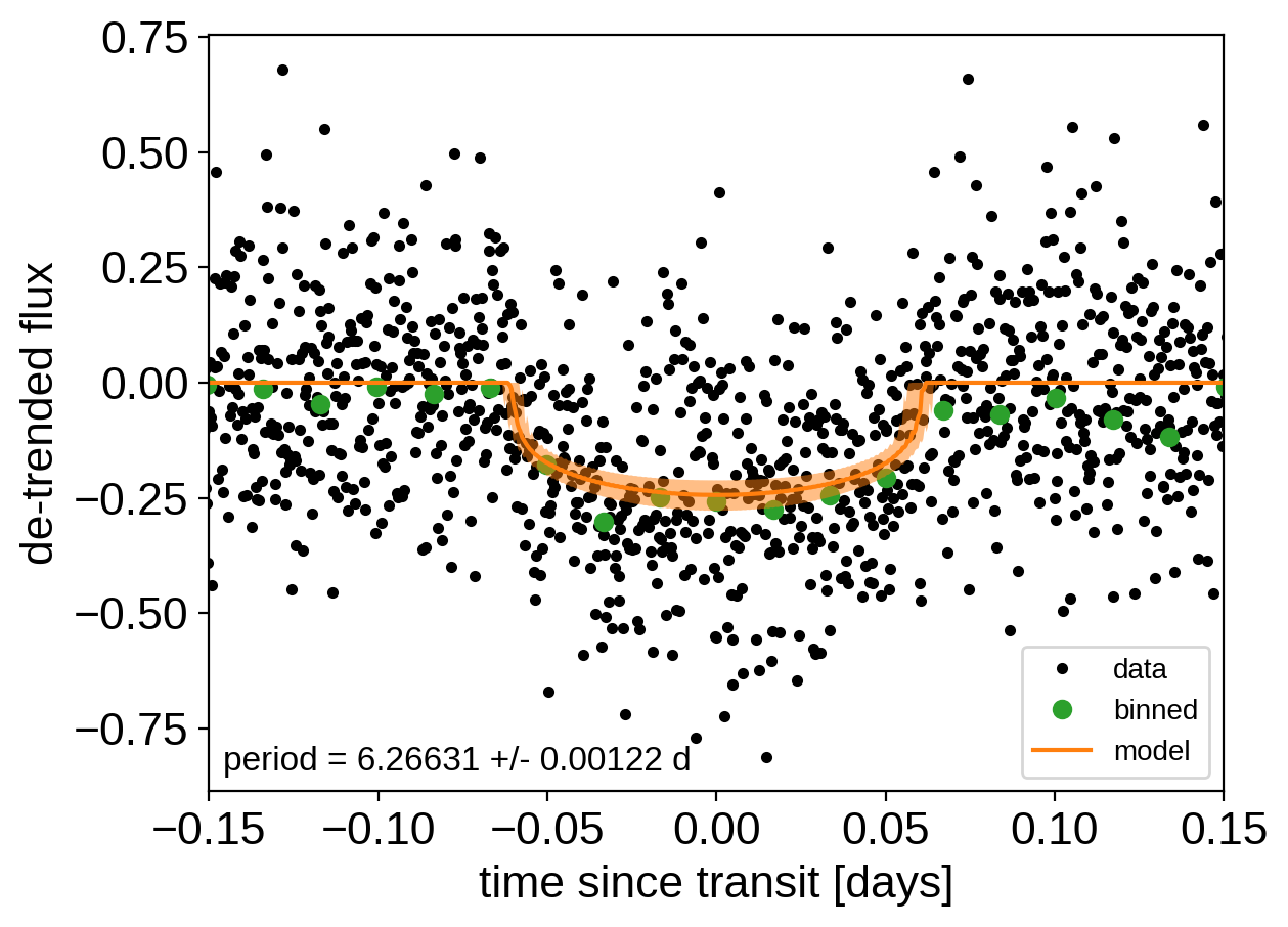
After sampling, we can make the usual plots. First, let’s look at the folded light curve plot:
[11]:
# Compute the GP prediction
gp_mod = np.median(trace["gp_pred"] + trace["mean"][:, None], axis=0)

# Get the posterior median orbital parameters
p = np.median(trace["period"])
t0 = np.median(trace["t0"])

# Plot the folded data
x_fold = (x[mask] - t0 + 0.5 * p) % p - 0.5 * p
plt.plot(x_fold, y[mask] - gp_mod, ".k", label="data", zorder=-1000)

# Overplot the phase binned light curve
bins = np.linspace(-0.41, 0.41, 50)
denom, _ = np.histogram(x_fold, bins)
num, _ = np.histogram(x_fold, bins, weights=y[mask])
denom[num == 0] = 1.0
plt.plot(
    0.5 * (bins[1:] + bins[:-1]), num / denom, "o", color="C2", label="binned"
)

# Plot the folded model
inds = np.argsort(x_fold)
inds = inds[np.abs(x_fold)[inds] < 0.3]
pred = trace["light_curves"][:, inds, 0]
pred = np.percentile(pred, [16, 50, 84], axis=0)
plt.plot(x_fold[inds], pred[1], color="C1", label="model")
art = plt.fill_between(
    x_fold[inds], pred[0], pred[2], color="C1", alpha=0.5, zorder=1000
)
art.set_edgecolor("none")

# Annotate the plot with the planet's period
txt = "period = {0:.5f} +/- {1:.5f} d".format(
    np.mean(trace["period"]), np.std(trace["period"])
)
plt.annotate(
    txt,
    (0, 0),
    xycoords="axes fraction",
    xytext=(5, 5),
    textcoords="offset points",
    ha="left",
    va="bottom",
    fontsize=12,
)

plt.legend(fontsize=10, loc=4)
plt.xlim(-0.5 * p, 0.5 * p)
plt.xlabel("time since transit [days]")
plt.ylabel("de-trended flux")
_ = plt.xlim(-0.15, 0.15)
And a corner plot of some of the key parameters:
[12]:
import corner
import astropy.units as u

varnames = ["period", "b", "ecc", "r_pl"]
samples = pm.trace_to_dataframe(trace, varnames=varnames)

# Convert the radius to Earth radii
samples["r_pl"] = (np.array(samples["r_pl"]) * u.R_sun).to(u.R_earth).value

_ = corner.corner(
    samples[["period", "r_pl", "b", "ecc"]],
    labels=[
        "period [days]",
        "radius [Earth radii]",
        "impact param",
        "eccentricity",
    ],
)

These all seem consistent with the previously published values.
As described in the citation tutorial, we can use citations.get_citations_for_model to construct an acknowledgement and BibTeX listing that includes the relevant citations for this model.
[13]:
with model:
    txt, bib = xo.citations.get_citations_for_model()
print(txt)
This research made use of \textsf{exoplanet} \citep{exoplanet} and its
dependencies \citep{celerite2:foremanmackey17, celerite2:foremanmackey18,
exoplanet:agol20, exoplanet:astropy13, exoplanet:astropy18,
exoplanet:exoplanet, exoplanet:kipping13, exoplanet:kipping13b,
exoplanet:luger18, exoplanet:pymc3, exoplanet:theano}.
[14]:
print("\n".join(bib.splitlines()[:10]) + "\n...")
@misc{exoplanet:exoplanet,
  author = {Daniel Foreman-Mackey and Rodrigo Luger and Ian Czekala and
            Eric Agol and Adrian Price-Whelan and Timothy D. Brandt and
            Tom Barclay and Luke Bouma},
   title = {exoplanet-dev/exoplanet v0.4.0},
   month = oct,
    year = 2020,
     doi = {10.5281/zenodo.1998447},
     url = {https://doi.org/10.5281/zenodo.1998447}
...