In this tutorial, we will reproduce the fits to the transiting planet in the Pi Mensae system discovered by Huang et al. (2018). The data processing and model are similar to the Putting it all together case study, but with a few extra bits like aperture selection and de-trending.
To start, we need to download the target pixel file:
[3]:
import numpy as np
import lightkurve as lk
import matplotlib.pyplot as plt
from astropy.io import fits

lc_file = lk.search_lightcurve(
    "TIC 261136679", sector=1, author="SPOC"
).download(quality_bitmask="hardest", flux_column="pdcsap_flux")
lc = lc_file.remove_nans().normalize().remove_outliers()
time = lc.time.value
flux = lc.flux
m = lc.quality == 0
with fits.open(lc_file.filename) as hdu:
    hdr = hdu[1].header

texp = hdr["FRAMETIM"] * hdr["NUM_FRM"]
texp /= 60.0 * 60.0 * 24.0

ref_time = 0.5 * (np.min(time) + np.max(time))
x = np.ascontiguousarray(time[m] - ref_time, dtype=np.float64)
y = np.ascontiguousarray(1e3 * (flux[m] - 1.0), dtype=np.float64)

plt.plot(x, y, ".k")
plt.xlabel("time [days]")
plt.ylabel("relative flux [ppt]")
_ = plt.xlim(x.min(), x.max())

Now, let’s use the box least squares periodogram from AstroPy (Note: you’ll need AstroPy v3.1 or more recent to use this feature) to estimate the period, phase, and depth of the transit.
[4]:
from astropy.timeseries import BoxLeastSquares

period_grid = np.exp(np.linspace(np.log(1), np.log(15), 50000))

bls = BoxLeastSquares(x, y)
bls_power = bls.power(period_grid, 0.1, oversample=20)

# Save the highest peak as the planet candidate
index = np.argmax(bls_power.power)
bls_period = bls_power.period[index]
bls_t0 = bls_power.transit_time[index]
bls_depth = bls_power.depth[index]
transit_mask = bls.transit_mask(x, bls_period, 0.2, bls_t0)

fig, axes = plt.subplots(2, 1, figsize=(10, 10))

# Plot the periodogram
ax = axes[0]
ax.axvline(np.log10(bls_period), color="C1", lw=5, alpha=0.8)
ax.plot(np.log10(bls_power.period), bls_power.power, "k")
ax.annotate(
    "period = {0:.4f} d".format(bls_period),
    (0, 1),
    xycoords="axes fraction",
    xytext=(5, -5),
    textcoords="offset points",
    va="top",
    ha="left",
    fontsize=12,
)
ax.set_ylabel("bls power")
ax.set_yticks([])
ax.set_xlim(np.log10(period_grid.min()), np.log10(period_grid.max()))
ax.set_xlabel("log10(period)")

# Plot the folded transit
ax = axes[1]
x_fold = (x - bls_t0 + 0.5 * bls_period) % bls_period - 0.5 * bls_period
m = np.abs(x_fold) < 0.4
ax.plot(x_fold[m], y[m], ".k")

# Overplot the phase binned light curve
bins = np.linspace(-0.41, 0.41, 32)
denom, _ = np.histogram(x_fold, bins)
num, _ = np.histogram(x_fold, bins, weights=y)
denom[num == 0] = 1.0
ax.plot(0.5 * (bins[1:] + bins[:-1]), num / denom, color="C1")

ax.set_xlim(-0.3, 0.3)
ax.set_ylabel("de-trended flux [ppt]")
_ = ax.set_xlabel("time since transit")

The transit model, initialization, and sampling are all nearly the same as the one in Putting it all together.
[5]:
import exoplanet as xo
import pymc3 as pm
import aesara_theano_fallback.tensor as tt

import pymc3_ext as pmx
from celerite2.theano import terms, GaussianProcess


def build_model(mask=None, start=None):
    if mask is None:
        mask = np.ones(len(x), dtype=bool)
    with pm.Model() as model:

        # Parameters for the stellar properties
        mean = pm.Normal("mean", mu=0.0, sd=10.0)
        u_star = xo.QuadLimbDark("u_star")

        # Stellar parameters from Huang et al (2018)
        M_star_huang = 1.094, 0.039
        R_star_huang = 1.10, 0.023
        BoundedNormal = pm.Bound(pm.Normal, lower=0, upper=3)
        m_star = BoundedNormal(
            "m_star", mu=M_star_huang[0], sd=M_star_huang[1]
        )
        r_star = BoundedNormal(
            "r_star", mu=R_star_huang[0], sd=R_star_huang[1]
        )

        # Orbital parameters for the planets
        t0 = pm.Normal("t0", mu=bls_t0, sd=1)
        log_period = pm.Normal("log_period", mu=np.log(bls_period), sd=1)
        log_r_pl = pm.Normal(
            "log_r_pl",
            sd=1.0,
            mu=0.5 * np.log(1e-3 * np.array(bls_depth))
            + np.log(R_star_huang[0]),
        )
        period = pm.Deterministic("period", tt.exp(log_period))
        r_pl = pm.Deterministic("r_pl", tt.exp(log_r_pl))
        ror = pm.Deterministic("ror", r_pl / r_star)
        b = xo.distributions.ImpactParameter("b", ror=ror)

        ecs = pmx.UnitDisk("ecs", testval=np.array([0.01, 0.0]))
        ecc = pm.Deterministic("ecc", tt.sum(ecs ** 2))
        omega = pm.Deterministic("omega", tt.arctan2(ecs[1], ecs[0]))
        xo.eccentricity.kipping13("ecc_prior", fixed=True, observed=ecc)

        # Transit jitter & GP parameters
        log_sigma_lc = pm.Normal(
            "log_sigma_lc", mu=np.log(np.std(y[mask])), sd=10
        )
        log_rho_gp = pm.Normal("log_rho_gp", mu=0, sd=10)
        log_sigma_gp = pm.Normal(
            "log_sigma_gp", mu=np.log(np.std(y[mask])), sd=10
        )

        # Orbit model
        orbit = xo.orbits.KeplerianOrbit(
            r_star=r_star,
            m_star=m_star,
            period=period,
            t0=t0,
            b=b,
            ecc=ecc,
            omega=omega,
        )

        # Compute the model light curve
        light_curves = pm.Deterministic(
            "light_curves",
            xo.LimbDarkLightCurve(u_star).get_light_curve(
                orbit=orbit, r=r_pl, t=x[mask], texp=texp
            )
            * 1e3,
        )
        light_curve = tt.sum(light_curves, axis=-1) + mean
        resid = y[mask] - light_curve

        # GP model for the light curve
        kernel = terms.SHOTerm(
            sigma=tt.exp(log_sigma_gp),
            rho=tt.exp(log_rho_gp),
            Q=1 / np.sqrt(2),
        )
        gp = GaussianProcess(kernel, t=x[mask], yerr=tt.exp(log_sigma_lc))
        gp.marginal("gp", observed=resid)
        pm.Deterministic("gp_pred", gp.predict(resid))

        # Fit for the maximum a posteriori parameters, I've found that I can get
        # a better solution by trying different combinations of parameters in turn
        if start is None:
            start = model.test_point
        map_soln = pmx.optimize(
            start=start, vars=[log_sigma_lc, log_sigma_gp, log_rho_gp]
        )
        map_soln = pmx.optimize(start=map_soln, vars=[log_r_pl])
        map_soln = pmx.optimize(start=map_soln, vars=[b])
        map_soln = pmx.optimize(start=map_soln, vars=[log_period, t0])
        map_soln = pmx.optimize(start=map_soln, vars=[u_star])
        map_soln = pmx.optimize(start=map_soln, vars=[log_r_pl])
        map_soln = pmx.optimize(start=map_soln, vars=[b])
        map_soln = pmx.optimize(start=map_soln, vars=[ecs])
        map_soln = pmx.optimize(start=map_soln, vars=[mean])
        map_soln = pmx.optimize(
            start=map_soln, vars=[log_sigma_lc, log_sigma_gp, log_rho_gp]
        )
        map_soln = pmx.optimize(start=map_soln)

    return model, map_soln


model0, map_soln0 = build_model()
optimizing logp for variables: [log_rho_gp, log_sigma_gp, log_sigma_lc]
message: Desired error not necessarily achieved due to precision loss.
logp: 362.5039496547183 -> 699.7041405471435
optimizing logp for variables: [log_r_pl]
message: Optimization terminated successfully.
logp: 699.7041405471435 -> 700.7459969464379
optimizing logp for variables: [b, log_r_pl, r_star]
message: Optimization terminated successfully.
logp: 700.7459969464379 -> 874.8144918463388
optimizing logp for variables: [t0, log_period]
message: Optimization terminated successfully.
logp: 874.8144918463443 -> 877.2071704947753
optimizing logp for variables: [u_star]
message: Optimization terminated successfully.
logp: 877.2071704947716 -> 877.6030372674369
optimizing logp for variables: [log_r_pl]
message: Optimization terminated successfully.
logp: 877.6030372674369 -> 877.6770071052002
optimizing logp for variables: [b, log_r_pl, r_star]
message: Optimization terminated successfully.
logp: 877.6770071052002 -> 877.7496031028384
optimizing logp for variables: [ecs]
message: Desired error not necessarily achieved due to precision loss.
logp: 877.7496031028384 -> 878.3326077642981
optimizing logp for variables: [mean]
message: Optimization terminated successfully.
logp: 878.3326077642981 -> 879.9061415287931
optimizing logp for variables: [log_rho_gp, log_sigma_gp, log_sigma_lc]
message: Optimization terminated successfully.
logp: 879.9061415287931 -> 880.0638635079661
optimizing logp for variables: [log_sigma_gp, log_rho_gp, log_sigma_lc, ecs, b, log_r_pl, log_period, t0, r_star, m_star, u_star, mean]
message: Desired error not necessarily achieved due to precision loss.
logp: 880.0638635079661 -> 935.2849116034062
Here’s how we plot the initial light curve model:
[6]:
def plot_light_curve(soln, mask=None):
    if mask is None:
        mask = np.ones(len(x), dtype=bool)

    fig, axes = plt.subplots(3, 1, figsize=(10, 7), sharex=True)

    ax = axes[0]
    ax.plot(x[mask], y[mask], "k", label="data")
    gp_mod = soln["gp_pred"] + soln["mean"]
    ax.plot(x[mask], gp_mod, color="C2", label="gp model")
    ax.legend(fontsize=10)
    ax.set_ylabel("relative flux [ppt]")

    ax = axes[1]
    ax.plot(x[mask], y[mask] - gp_mod, "k", label="de-trended data")
    for i, l in enumerate("b"):
        mod = soln["light_curves"][:, i]
        ax.plot(x[mask], mod, label="planet {0}".format(l))
    ax.legend(fontsize=10, loc=3)
    ax.set_ylabel("de-trended flux [ppt]")

    ax = axes[2]
    mod = gp_mod + np.sum(soln["light_curves"], axis=-1)
    ax.plot(x[mask], y[mask] - mod, "k")
    ax.axhline(0, color="#aaaaaa", lw=1)
    ax.set_ylabel("residuals [ppt]")
    ax.set_xlim(x[mask].min(), x[mask].max())
    ax.set_xlabel("time [days]")

    return fig


_ = plot_light_curve(map_soln0)

As in Putting it all together, we can do some sigma clipping to remove significant outliers.
[7]:
mod = (
    map_soln0["gp_pred"]
    + map_soln0["mean"]
    + np.sum(map_soln0["light_curves"], axis=-1)
)
resid = y - mod
rms = np.sqrt(np.median(resid ** 2))
mask = np.abs(resid) < 5 * rms

plt.figure(figsize=(10, 5))
plt.plot(x, resid, "k", label="data")
plt.plot(x[~mask], resid[~mask], "xr", label="outliers")
plt.axhline(0, color="#aaaaaa", lw=1)
plt.ylabel("residuals [ppt]")
plt.xlabel("time [days]")
plt.legend(fontsize=12, loc=3)
_ = plt.xlim(x.min(), x.max())

And then we re-build the model using the data without outliers.
[8]:
model, map_soln = build_model(mask, map_soln0)
_ = plot_light_curve(map_soln, mask)
optimizing logp for variables: [log_rho_gp, log_sigma_gp, log_sigma_lc]
message: Optimization terminated successfully.
logp: 2218.3946388346744 -> 2324.6549089775276
optimizing logp for variables: [log_r_pl]
message: Optimization terminated successfully.
logp: 2324.6549089775276 -> 2324.6704028177396
optimizing logp for variables: [b, log_r_pl, r_star]
message: Optimization terminated successfully.
logp: 2324.6704028177396 -> 2324.672908017927
optimizing logp for variables: [t0, log_period]
message: Desired error not necessarily achieved due to precision loss.
logp: 2324.6729080179307 -> 2324.677011630767
optimizing logp for variables: [u_star]
message: Optimization terminated successfully.
logp: 2324.6770116307653 -> 2324.7453217567536
optimizing logp for variables: [log_r_pl]
message: Optimization terminated successfully.
logp: 2324.7453217567536 -> 2324.7453263316966
optimizing logp for variables: [b, log_r_pl, r_star]
message: Optimization terminated successfully.
logp: 2324.7453263316966 -> 2324.748426822599
optimizing logp for variables: [ecs]
message: Optimization terminated successfully.
logp: 2324.748426822599 -> 2324.7484421673366
optimizing logp for variables: [mean]
message: Optimization terminated successfully.
logp: 2324.7484421673366 -> 2324.756210519281
optimizing logp for variables: [log_rho_gp, log_sigma_gp, log_sigma_lc]
message: Optimization terminated successfully.
logp: 2324.756210519281 -> 2324.756483895066
optimizing logp for variables: [log_sigma_gp, log_rho_gp, log_sigma_lc, ecs, b, log_r_pl, log_period, t0, r_star, m_star, u_star, mean]
message: Desired error not necessarily achieved due to precision loss.
logp: 2324.756483895066 -> 2324.7573304646853

Now that we have the model, we can sample:
[9]:
np.random.seed(261136679)
with model:
    trace = pmx.sample(
        tune=2500,
        draws=2000,
        start=map_soln,
        cores=2,
        chains=2,
        initial_accept=0.8,
        target_accept=0.95,
        return_inferencedata=True,
    )
Multiprocess sampling (2 chains in 2 jobs)
NUTS: [log_sigma_gp, log_rho_gp, log_sigma_lc, ecs, b, log_r_pl, log_period, t0, r_star, m_star, u_star, mean]
Sampling 2 chains for 2_500 tune and 2_000 draw iterations (5_000 + 4_000 draws total) took 2143 seconds.
There were 10 divergences after tuning. Increase `target_accept` or reparameterize.
The number of effective samples is smaller than 25% for some parameters.
[10]:
import arviz as az
[11]:
az.summary(
    trace,
    var_names=[
        "omega",
        "ecc",
        "r_pl",
        "b",
        "t0",
        "period",
        "r_star",
        "m_star",
        "u_star",
        "mean",
    ],
)
[11]:
| mean | sd | hdi_3% | hdi_97% | mcse_mean | mcse_sd | ess_bulk | ess_tail | r_hat | |
|---|---|---|---|---|---|---|---|---|---|
| omega | 0.412 | 1.783 | -2.785 | 3.128 | 0.040 | 0.029 | 2080.0 | 3205.0 | 1.00 |
| ecc | 0.231 | 0.173 | 0.001 | 0.532 | 0.013 | 0.012 | 431.0 | 132.0 | 1.01 |
| r_pl | 0.016 | 0.001 | 0.014 | 0.019 | 0.000 | 0.000 | 2248.0 | 1654.0 | 1.00 |
| b | 0.457 | 0.219 | 0.000 | 0.762 | 0.006 | 0.004 | 1089.0 | 743.0 | 1.00 |
| t0 | -13.730 | 0.003 | -13.736 | -13.723 | 0.000 | 0.000 | 2282.0 | 2009.0 | 1.00 |
| period | 6.266 | 0.001 | 6.264 | 6.269 | 0.000 | 0.000 | 3356.0 | 2351.0 | 1.01 |
| r_star | 1.099 | 0.023 | 1.055 | 1.141 | 0.000 | 0.000 | 3509.0 | 2761.0 | 1.00 |
| m_star | 1.094 | 0.040 | 1.020 | 1.164 | 0.001 | 0.000 | 4075.0 | 2861.0 | 1.00 |
| u_star[0] | 0.563 | 0.365 | 0.001 | 1.184 | 0.008 | 0.006 | 1888.0 | 1711.0 | 1.00 |
| u_star[1] | 0.158 | 0.393 | -0.528 | 0.854 | 0.010 | 0.007 | 1509.0 | 2511.0 | 1.00 |
| mean | 0.021 | 0.012 | -0.002 | 0.044 | 0.000 | 0.000 | 2150.0 | 1707.0 | 1.00 |
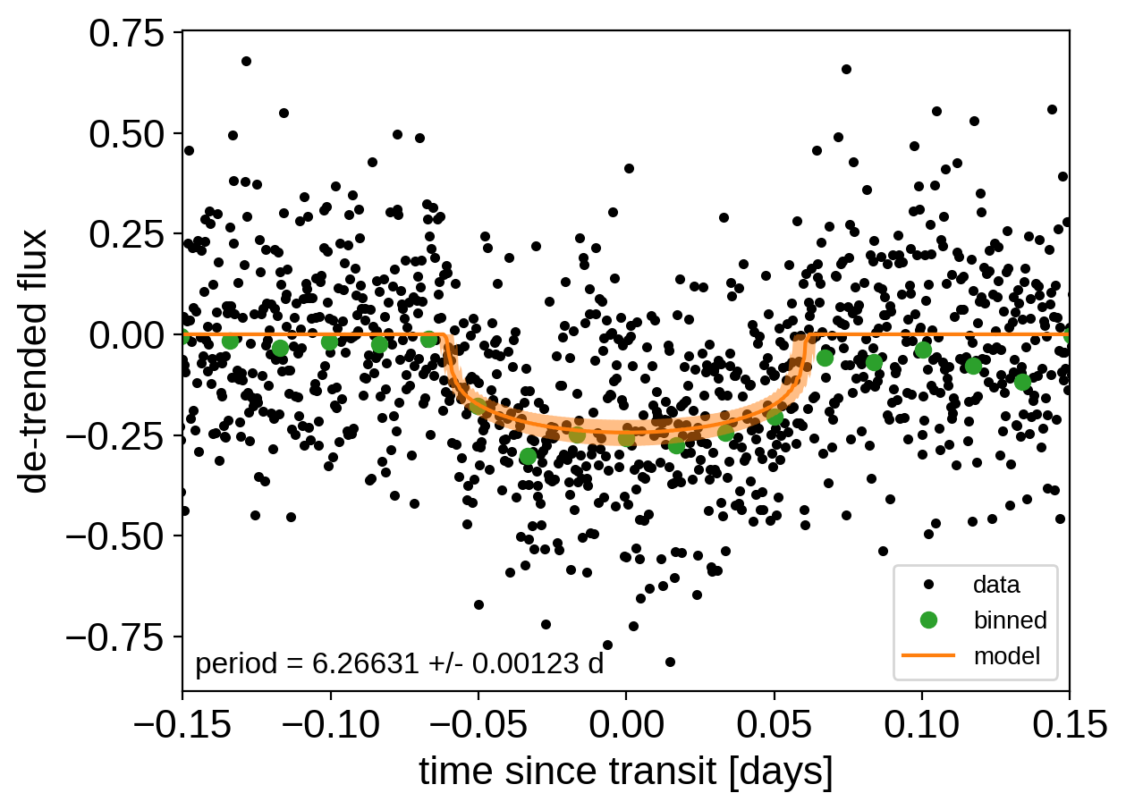
After sampling, we can make the usual plots. First, let’s look at the folded light curve plot:
[12]:
flat_samps = trace.posterior.stack(sample=("chain", "draw"))

# Compute the GP prediction
gp_mod = np.median(
    flat_samps["gp_pred"].values + flat_samps["mean"].values[None, :], axis=-1
)

# Get the posterior median orbital parameters
p = np.median(flat_samps["period"])
t0 = np.median(flat_samps["t0"])

# Plot the folded data
x_fold = (x[mask] - t0 + 0.5 * p) % p - 0.5 * p
plt.plot(x_fold, y[mask] - gp_mod, ".k", label="data", zorder=-1000)

# Overplot the phase binned light curve
bins = np.linspace(-0.41, 0.41, 50)
denom, _ = np.histogram(x_fold, bins)
num, _ = np.histogram(x_fold, bins, weights=y[mask])
denom[num == 0] = 1.0
plt.plot(
    0.5 * (bins[1:] + bins[:-1]), num / denom, "o", color="C2", label="binned"
)

# Plot the folded model
inds = np.argsort(x_fold)
inds = inds[np.abs(x_fold)[inds] < 0.3]
pred = np.percentile(
    flat_samps["light_curves"][inds, 0], [16, 50, 84], axis=-1
)
plt.plot(x_fold[inds], pred[1], color="C1", label="model")
art = plt.fill_between(
    x_fold[inds], pred[0], pred[2], color="C1", alpha=0.5, zorder=1000
)
art.set_edgecolor("none")

# Annotate the plot with the planet's period
txt = "period = {0:.5f} +/- {1:.5f} d".format(
    np.mean(flat_samps["period"].values), np.std(flat_samps["period"].values)
)
plt.annotate(
    txt,
    (0, 0),
    xycoords="axes fraction",
    xytext=(5, 5),
    textcoords="offset points",
    ha="left",
    va="bottom",
    fontsize=12,
)

plt.legend(fontsize=10, loc=4)
plt.xlim(-0.5 * p, 0.5 * p)
plt.xlabel("time since transit [days]")
plt.ylabel("de-trended flux")
_ = plt.xlim(-0.15, 0.15)
And a corner plot of some of the key parameters:
[13]:
import corner
import astropy.units as u

trace.posterior["r_earth"] = (
    trace.posterior["r_pl"].coords,
    (trace.posterior["r_pl"].values * u.R_sun).to(u.R_earth).value,
)

_ = corner.corner(
    trace,
    var_names=["period", "r_earth", "b", "ecc"],
    labels=[
        "period [days]",
        "radius [Earth radii]",
        "impact param",
        "eccentricity",
    ],
)

These all seem consistent with the previously published values.
As described in the citation tutorial, we can use citations.get_citations_for_model to construct an acknowledgement and BibTeX listing that includes the relevant citations for this model.
[14]:
with model:
    txt, bib = xo.citations.get_citations_for_model()
print(txt)
This research made use of \textsf{exoplanet} \citep{exoplanet} and its
dependencies \citep{celerite2:foremanmackey17, celerite2:foremanmackey18,
exoplanet:agol20, exoplanet:arviz, exoplanet:astropy13, exoplanet:astropy18,
exoplanet:exoplanet, exoplanet:kipping13, exoplanet:kipping13b,
exoplanet:luger18, exoplanet:pymc3, exoplanet:theano}.
[15]:
print("\n".join(bib.splitlines()[:10]) + "\n...")
@misc{exoplanet:exoplanet,
  author = {Daniel Foreman-Mackey and Arjun Savel and Rodrigo Luger and
            Ian Czekala and Eric Agol and Adrian Price-Whelan and
            Christina Hedges and Emily Gilbert and Tom Barclay and Luke Bouma
            and Timothy D. Brandt},
   title = {exoplanet-dev/exoplanet v0.4.5},
   month = mar,
    year = 2021,
     doi = {10.5281/zenodo.1998447},
...